![]()
The Hall Effect Gaussmeter
|
Hall effect gaussmeters are used in research, product design, education, and materials inspection. A better understanding of magnetic fields and the Hall effect will help the operator get the most out of these instruments. John Boettger, F.W. Bell |
|
1 Wb = 108 Mx
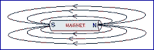
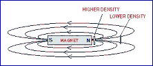
Figure 1 depicts a simple bar magnet with two poles. Faraday viewed the pole faces as containing thousands of smaller unit poles and the space surrounding the magnet as filled with the same number of flux lines, one line connecting each north-south pair. Flux lines are generally viewed as exiting the north pole and returning to the south pole. The total number of flux lines passing perpendicularly through a given area is called flux density, B, or magnetic induction.
|
1 T = 10,000 G
The force within the magnet that produces the flux lines is the magnetic field strength, H, or magnetizing force. In the CGS system, one oersted (Oe) is produced when two like poles of two identical magnets, placed one centimeter apart, cause a repelling force of one dyne. The SI system assumes an infinitely long coil of wire (solenoid) wound with a number of turns per meter and carrying one amp of current. The magnetic field strength at the center of the solenoid is given in amps per meter, or A/m. The relationship between oersted and A/m is:
1 A/m = 79.58 Oe
It must be understood that flux density and magnetic field strength are related but not equal. The intrinsic characteristics of the magnetic material must be considered. Only in free space (air) are flux density and field strength considered equal.
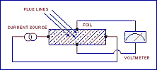
The Hall EffectIn the 19th century Edwin Hall attached a wire to each side of a rectangular piece of gold foil (see Figure 2), passed an electrical current through the length of the foil, and measured the voltage across the width of the foil.
|
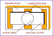
A modern Hall effect device (see Photo 1), commonly called a Hall generator, consists of a thin square or rectangular plate or film of GaAs or InAs to which four electrical contacts are made (see Figure 3).
|
The output of a Hall device is greatest when the flux lines are perpendicular to the surface of the material. When the angle is held constant, and a constant current is provided through the material, the Hall voltage is directly proportional to flux density. Conversely, holding the flux density and current constant allows the device to respond to the angle of the flux lines. One particularly useful aspect of a Hall generator is its ability to sense the direction of flux travel, allowing it to detect both static (DC) and alternating (AC) fields.
The active area, the area of greatest magnetic sensitivity, is considered to be located in the center of the plate or film and is the largest circular area that can fit within the boundary of the connection points. Present manufacturing methods have produced active areas as small as 0.13 mm in dia. Some devices are only 0.25 mm thick, allowing their use in very tight spaces.
The ideal Hall generator produces zero voltage in the absence of a magnetic field, but actual devices are subject to variations in materials and construction. Most Hall generators therefore produce some initial output in a zero field. This signal, known as the Hall offset voltage, Vm, can be canceled with external analog circuitry, arithmetically canceled by a computer, or removed by abrasive or laser trimming. The offset voltage is affected by temperature and can change in either the positive or negative direction. Vm is usually specified as a maximum ±µV/ºC change.
The ideal Hall generator has a constant sensitivity over a range of flux density, but actual devices are seldom linear. Typical accuracy ranges from ±0.1% to ±2% of reading. The sensitivity is also temperature dependent and always decreases as temperature increases for both GaAs and InAs. Typical values range from 0.04%/ºC to 0.2%/ºC.
A Hall generator produces a positive voltage for flux lines traveling in one direction and a negative voltage in the opposite direction. Ideally, for equal fields of opposite polarity a Hall device will generate equal voltages of opposite polarity. In reality there is a phenomenon called a reversibility error that causes these voltages to be slightly different in magnitude. This is caused, in part, by inconsistencies in the material's composition and by the locations and sizes of the electrical connections to the edges of the Hall plate. The error is usually stated in terms of percent of reading and can be as high as 1%.
A Hall generator's accuracy when sensing high-frequency AC magnetic fields is primarily limited by the connections to the Hall material rather than by the material itself. Inductive wiring loops within a changing magnetic field generate significant voltages on their own, sometimes higher than the Hall voltage. Careful design is required to reduce this effect to a minimum. (The Hall generator was also discussed in "Understanding Hall Effect Devices," Bill Drafts, Sensors, September 1997.)
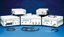
The Hall Effect Gaussmeter and ProbeA Hall generator may produce signals as low as 500 nV/G or as high as 200 µV/G. Hall effect gaussmeters (or teslameters) are designed to amplify and condition these low-level signals and provide a result that is calibrated in terms of gauss and/or tesla. These instruments range from small handheld meters to more sophisticated bench-type units (see Photo 2).
|
Often the Hall generator is mounted inside a protective tube, or stem, made of aluminum, fiberglass or other nonmagnetic material. The wires are connected internally to a flexible cable and the cable is terminated with a multipin connector. This assembly, known as a Hall probe, is generally available in two configurations (see Figure 4).
|

The Hall effect is generally considered as having a maximum resolution of 1 mG (100 nT). Below this level, electrical noise and thermal effects swamp the usable signal.
|

Gaussmeters are nearly as easy to use as voltmeters, but there are several sources of errors that can affect accuracy if the operator is not familiar with the Hall effect or magnetic fields.
"Zeroing" or "nulling" the Hall probe and meter is one of the most important steps toward obtaining accurate flux density measurements. As stated earlier, most Hall devices produce an offset signal in the absence of a magnetic field. Second, the internal circuitry of the meter itself is likely to produce a small offset signal even in the absence of an input signal. Finally, local flux from the Earth (~0.5 G) or nearby magnetic sources will affect the Hall sensor. The process of zeroing eliminates these errors.
|
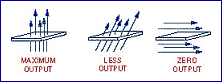
Another common source of error is due to the angle of the Hall generator relative to the flux being measured. As shown in Figure 6, the highest output is generated when the flux lines are perpendicular to the Hall sensor. This is the way each Hall probe is calibrated and specified. It is often incorrectly assumed that the plane of the Hall generator is exactly the same as the axis of the probe's stem, but because of variations in material and manufacturing this alignment is not a certainty. The user should always peak the probe, a process in which the probe is rotated and tilted in several planes to obtain the highest possible output for a given field. At that point the probe should be fixed in place.
|
|

Many gaussmeter manufacturers also offer a variety of permanent reference magnets and reference coils that can be used to verify the basic operation of the equipment. Verifying overall accuracy often requires a huge investment in magnetic standards and specialized equipment, so certification and calibration are often left to the original manufacturer or a third-party calibration lab. Most manufacturers recommend a one-year calibration cycle.
Hall effect gaussmeters provide an economical and relatively easy way to measure flux density. They are used in research, product design, education, and materials inspection. A better understanding of magnetic fields and the Hall effect will lead to more effective use of these instruments.
| Magnetism: An Historical Perspective
The first recorded observations of magnetism occurred in the district of Magnesia, Thessaly, around 600 BC. Naturally occurring stones found in this region had unusual properties. They were attracted to iron but not to most other materials. Two stones might either be attracted to or repel each other. An iron needle touched by a stone would itself behave like the stone. If the stone or needle were freely suspended it would always orient itself to the same point on Earth. Thus the compass was one of the first practical devices based on magnetism, guiding the traveler as did a guiding star, or lodestar. The lodestone (magnetite, Fe3O4) derived its name from this analogy (lode meant way in Middle English), and the term magnet evolved from the district's name, Magnesia. In 1269 Frenchmen Peter Peregrinus and Pierre de Maricourt, using a compass and a spherical lodestone, determined the existence of invisible lines of force surrounding the sphere just as the meridian lines surround the Earth, converging at points at opposite ends of the sphere. Maricourt called these points the north pole and south pole and noted that the force was always strongest at these points. Subsequent research found that magnetic poles always occur in pairs–if a lodestone is broken into many pieces, each piece will have a new set of poles. In 1600 William Gilbert performed the first great systematic study of magnetism. Some of his most important work focused on terrestrial magnetism, and demonstrated that the Earth itself is a large magnet. At that time magnets were primarily used to lift heavy iron objects. Gilbert developed better ways to produce strong magnets, but the only magnetizing forces available at that time were other lodestones and the Earth. Major breakthroughs came in 1820 when Oersted proved a relationship between magnetism and electricity, and in 1825 when Sturgeon invented the electromagnet. Magnetic fields could now be generated at will and at intensities much stronger than any permanent magnet. These discoveries led Faraday to develop his theories on electromagnetic induction, which led to the development of the transformer, the alternator, and the dynamo. These inventions retired the chemical battery as man's primary source of electric current and led to the development of today's electric lights, television, audio speakers, credit cards, electric motors, toys, disk drives, medical imaging, levitated rail systems, and other wonders. |
John Boettger is Design Engineering Manager, F.W. Bell, Division of Bell Technologies Inc., 6120 Hanging Moss Rd., Orlando, FL 32807; 407-678-6900, x-237, fax 407-677-5765.
